Interpretable AI For Better Operationalization: A Case For Constrained Regression

Author: Kaushik Bar, CTO & Chief Data Scientist, Inxite Out

Interpretable AI for better Operationalization: A case for Constrained Regression

How often do you find that a major chunk of the business knowledge of your domain experts goes in vain because your data science team cannot incorporate those into their AI models? How often do your AI models fail to get operationalized due to the lack of trust of the business stakeholders in your model’s outputs?

Let’s face it – no model is perfect. Every model approximates the underlying data in its bid to achieve generalization. And no real-world data is without imperfections. Sometimes, subtle data imperfections can lead to results that look decently accurate overall but make no business sense after deployment at the time of consumption and acting upon it.

In this article, we will take up a very common and simple business scenario involving MLR (Multiple Linear Regression), point out its limitations in capturing the complexity of the underlying business dynamics, and finally discuss how a special technique called Constrained Regression can allow us to include prior business knowledge and complex business constraints into the model, enabling more interpretable and operationalizable solution.

How to solve Constrained Regression problem?

In Constrained Regression, the optimization (minimization of error) happens in an iterative manner (subject to termination conditions based on pre-set tolerance levels), unlike the traditional linear regression. One of the popular methods to solve the optimization problem in Constrained Regression is TRF (Trust Region Reflective) algorithm.

Why not Simplex?

In operations research, Dantzig’s simplex method is a popular algorithm for several types of optimizations subject to constraints. However, it operates on linear programs and typically finds the optimal solution(s) in one of the vertices of the polytope it defines as the feasible region. Constrained Regression on the other hand deals with non-linear least squares problem and is not necessarily guaranteed to find solution at the boundaries of feasible regions. Hence Simplex and its variants are not suitable for this purpose.

Why not Gradient Descent?

Gauss–Newton (GN) algorithm is considered as the reference method for nonlinear least squares problems. The basic GN method has quadratic convergence close to the solution if certain assumptions on the residuals are valid (linear approximation and sufficient proximity to zero). To meet these conditions, two major versions of the GN algorithm came into existence: Line Search and Trust Region.

Modified from Original Image: David Mark from Pixabay

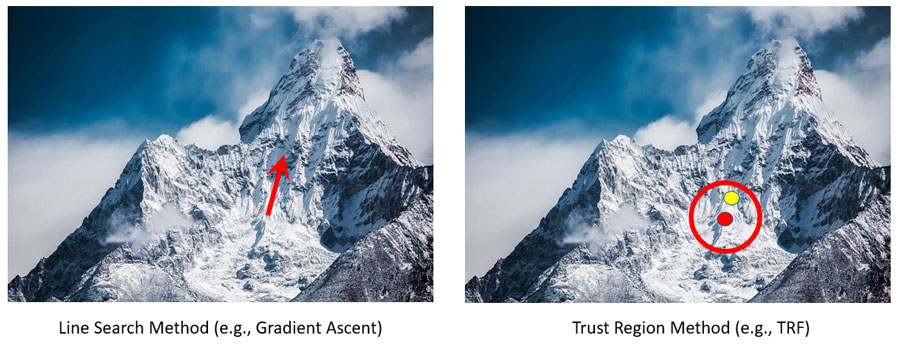
Gradient descent is a line search method. We determine the descending direction first and then we take a step in that direction. In gradient descent, step size = gradient * learning rate.

TRF on the other hand is a trust region method. We determine the maximum step size that we want to explore and then we locate the optimal point within that trust region. The trust region can be expanded or shrunk in runtime to adjust to the curvature of the surface.

TRF tends to work better than gradient descent in low data volume scenarios. However, gradient descent converges faster than TRF when there is a large volume of data to train on.

What is TRF?

TRF algorithm works by first defining a region called the Trust Region (TR). The size of the TR is usually defined by the radius in Euclidean norm. It is an iterative method, and convergence happens if the region is convex.

A TR is a subset of the region of the objective function that is to some extent approximated by a model function (often a quadratic). TRF then takes a step forward within the region. If a notable decrease (for minimization problems) is gained after the step forward, then the model is believed to be a good representation of the original objective function, and therefore the region is expanded.

If the improvement is too subtle or negative, the model is not to be believed as a good representation of the original objective function within that region, and therefore the region is contracted. The fit is evaluated by comparing the ratio of expected improvement from the model approximation with the actual improvement observed in the objective function. Simple thresholding of the ratio is used as the criterion for expansion and contraction.

Application in a business scenario

Let us take for an example the automation of operational expenditure forecasting. For a large organization, a major chunk of the efforts in such a business problem will involve forecasting of the wage costs many months in advance for several hundreds of cost centres involving many different functions across the globe. Wage rates are sensitive information, and hence might not be available. What we might have instead could be the historical total wage costs for any given cost centre, and the aggregated headcounts (historical and planned) across several wage groups in that cost centre. The linear relationship existing in the data can be leveraged to implement an MLR-based Wage Model to predict the approximate average salary spends per wage group.

However, the natural data imperfections may lead to situations where the wage rates predicted by the MLR model may not adhere to business criteria governing the wage rates among different wage groups. This would result in lack of interpretability and trust on the model.

Let us consider a few common business constraints a typical wage model must adhere to:

• Pre-defined order among the wages across different workgroups based on seniority.
• Minimum pre-defined gaps in between the average wage slabs across these groups.
• Upper and lower (greater than zero) bounds for each wage group.

To incorporate these business criteria, we need inequality constraints on regression coefficients, which linear regression does not allow. Linear regression is an unconstrained method. It does not incorporate any constraints on the coefficients and may lead to incorrect / unexplainable regression coefficients.

Examples of more business scenarios where Constrained Regression might help

The example of Wage Model described in this article is not the only business scenario where Constrained Regression would help. Consider for example that you know that Covid impacted the travelling expenses in your business over the last 2 years negatively, but you expect things to bounce back soon – and yet your AI model is not able to capture such relationships due to data insufficiency. Or, you know that the effectiveness of one of your promotional channels is at least 1.5X more compared to another, and yet your AI model is failing to capture this intuition in the results. Constrained Regression can help in each of these cases immensely.

Conclusion

For any AI model, accuracy is just one of the metrics that businesses rely upon. It is not the only metric. Lack of interpretability and trustworthiness of AI models can significantly impact the adoption rate of AI models. This is where Constrained Regression can help.

Despite its simplicity, linear regression plays an important role in modelling and interpreting data relationships in many business scenarios of today. Yet there is a general lack of availability of off-the-shelf tools to incorporate various commonly occurring business constraints while applying these models. The practitioners of data science can add Constrained Regression to their arsenal of tools for including prior business knowledge in their regression models and make their AI solutions more business aware.

(Featured Image Courtesy: S. Hermann & F. Richter, Pixabay)